Molecular graph learning in the Optimal Transport Geometry
- Introduction
- Chemistry basics
- Prior work
- Graph encoder
- Graph decoder - Issues
- Optimal Transport intro
- Graph decoder - Dictionary learning idea
- Graph decoder - Dictionary learning point clouds
- Graph decoder - From pointcloud to discrete graph
- Experiments
- Attempt at a downstream task
- Future work idea - improving the Tanimoto similarity
- Conclusion
- References
Introduction #
What #
This blog post is short article about my master thesis “Molecular Graph Learning in the Optimal Transport Geometry” done at ETH Zurich under the supervision of Prof. Thomas Hofmann (ETH), Dr. Octavian Ganea (MIT) and Dr. Gary Bécigneul (ETH) (10/10/2020). Parts of this work were collaborative with Octav Dragoi (TUM) who was working on “Optimizing Molecular Graphs in the Wasserstein Space”. In this work, we are concerned with learning a latent space for molecular graphs and define a geometry to measure distances between molecules using Optimal Transport (OT). This latent space can be later used for downstream tasks such as generating molecules, property prediction or molecule optimization.
Why #
In traditional computer-aided drug design (CADD), molecules formed with hand-crafted bond rules are enumerated and evaluated against some property of interest (e.g. obtaining more potent drugs with fewer side effects). While this technique has the advantage that it leaves us with knowledge of how to synthesize a molecule, it’s an untargeted search over a small subspace of the gigantic chemical space that remains vastly unexplored.
More recent developments on CADD that use machine learning techniques $\href{#3}{[3]} \href{#4}{[4]} \href{#5}{[5]}$, focus largely on learning a mapping from the discrete chemical space to a continuous lower-dimensional space and vice versa. This continuous latent space allows for downstream tasks such as molecular generation, optimization and property prediction.
Chemistry basics #
In this work we model molecules as graphs with node attributes (e.g. atom type - Carbon/Oxygen/.., charge etc) and edge attributes (e.g. bond type - single/double/triple bond, depth etc). To use this abstraction we need to understand what constraints are necessary for a molecular graph to be a semantically valid molecule e.g. a carbon with $0$ charge can form up to $4$ bonds. Note that this is a simplification of reality (e.g. hypervalent atoms don’t follow the standard valency rules), but it’s common practice in chemoinformatics (e.g. see RDKit $\href{#6}{[6]}$).
For chemistry-inclined audience, we are working with organic compounds with covalent bonds and charged atoms are formed using a solvent / dilution. All the molecules considered are in “Kekulized” form (we assign bond orders to aromatic bonds s.t. the valence constraints are satisfied) with Hydrogens removed.
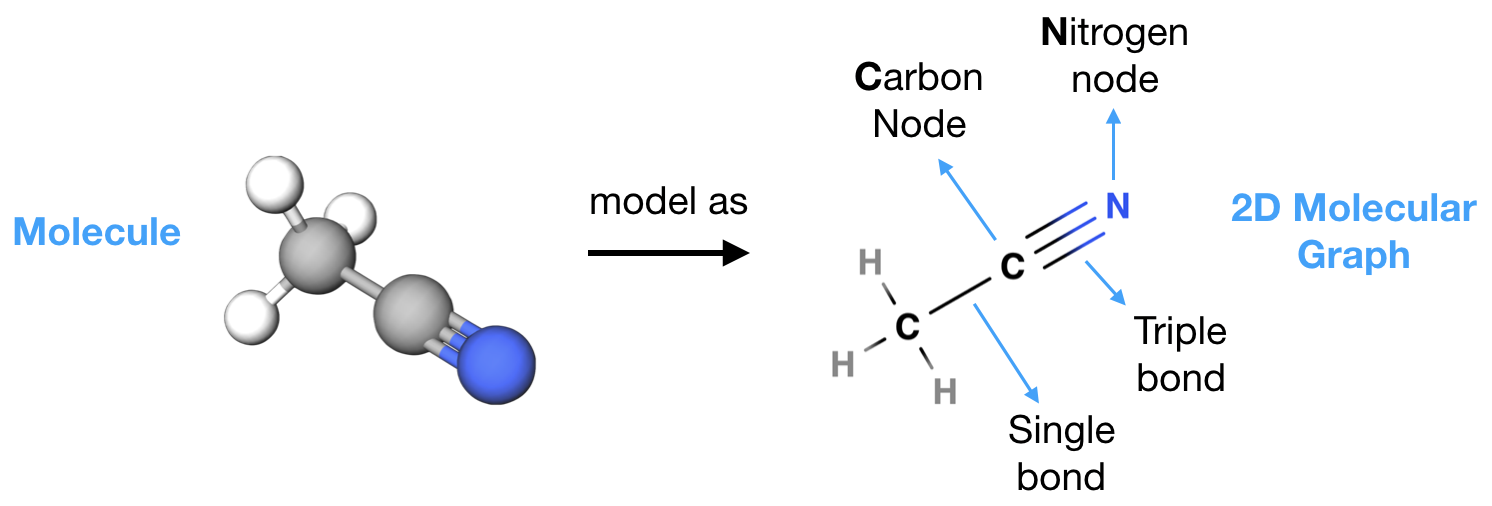
For a molecular graph to be semantically valid we require:
- Connectivity constraint: single connected component
- Valence constraint: degree constraint for every atom in the molecule e.g. Carbon (C) up to $4$ bonds, Nitrogen (N) up to $3$ etc
Additionally, to compare with the generated molecules we use the following chemically-aware metrics:
- Tanimoto similarity coefficient $\href{#1}{[1]}$: Chemical property similarity measure, uses Morgan fingerprints
- FCD $\href{#2}{[2]} \href{#28}{[28]}$: Measures how close $2$ molecular distributions are, using pertained latent representations of molecules
Prior work #
We do a quick review of prior work that learns a latent space for molecules for generation, optimization and property prediction. In generation they model the distribution of the latent space, in optimization they optimize on the latent space w.r.t. some property and in property prediction they use the latent space to get pertained embeddings.
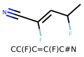
String representations of moleculels (SMILES, SELFIES) #
Represent molecules as strings using some parsing algorithm on top of the molecular graph $\href{#16}{[16]} \href{#17}{[17]} \href{#18}{[18]} \href{#19}{[19]} \href{#20}{[20]}$.
Pros/Cons:
- (+) Re-use SOTA NLP methods
- (-) String representations are not designed to capture molecular similarity, chemically similar molecules can have very different string representations
- (-) Seq2Seq / Transformer methods on top of strings are not permutation invariant w.r.t. graph nodes
Autoregressive approaches #
Autoregressive approaches operate on graphs. They assume a node or edge ordering and encode/decode molecules according to the ordering $\href{#21}{[21]} \href{#22}{[22]} \href{#23}{[23]} \href{#24}{[24]}$.
Pros/Cons:
- (+) Can always generate valid molecules by filtering the allowed actions at each step
- (-) Not permutation invariant w.r.t. graph nodes
- (-) Problematic for big molecules (hard to model long-term dependencies)

Junction Tree models #
Junction tree models $\href{#26}{[26]} \href{#4}{[4]}$ assume a fixed vocabulary of building blocks which can be combined to construct graphs. Encoding / decoding involves $2$ steps: the tree structured skeleton of the molecule, the subgraph that is represented by each node in the tree graph.
Pros/Cons:
- (+) Can enforce validity by filtering the predicted subgraphs
- (+) Can model bigger molecules easier than autoregressive approaches
- (-) Unclear what is the best vocabulary of subgraphs + limits the expressiveness of the model
- (-) Junction tree not unique and not guaranteed to exist
- (-) No permutation and isomorphism invariance
![Junction tree approach. The clusters (colored circles) are selected from a fixed vocabulary and are abstracted away, to form the Junction tree. Both the molecular graph and the Junction tree are separately encoded. The Junction tree is the first to be decoded. The decoded junction tree is combined with the molecular graph hidden representation to decode the clusters sequentially, selecting only the ones that will keep the molecule valid. Image taken from $\href{#4}{[4]}$](../../../assets/images/molgraphlearning/jt.png)
Our approach #
Desired inductive biases:
- Permutation and isomorphism invariance w.r.t. graph nodes
- Decode semantically valid molecules
- No fixed vocabulary
- Operate on graphs
To achieve this we perform one-shot prediction (from the latent representation to the graph), without introducing an ordering of the nodes. A big issue this method can have is that when nodes and edges are predicted jointly at once (needed for permutation and isomorphism invariance), generated graphs can be invalid e.g. disconnected graph.

Note: Regularized VAE $\href{#11}{[11]}$ also generates valid molecules in one-shot by expressing discrete constraints in a differentiable manner. However, they achieve very low validity $34.9\%$ and their approach is not permutation invariant (because of their loss function). We compare this with our approach in the $\href{#experiments}{Experiments}$ section.
Graph encoder #
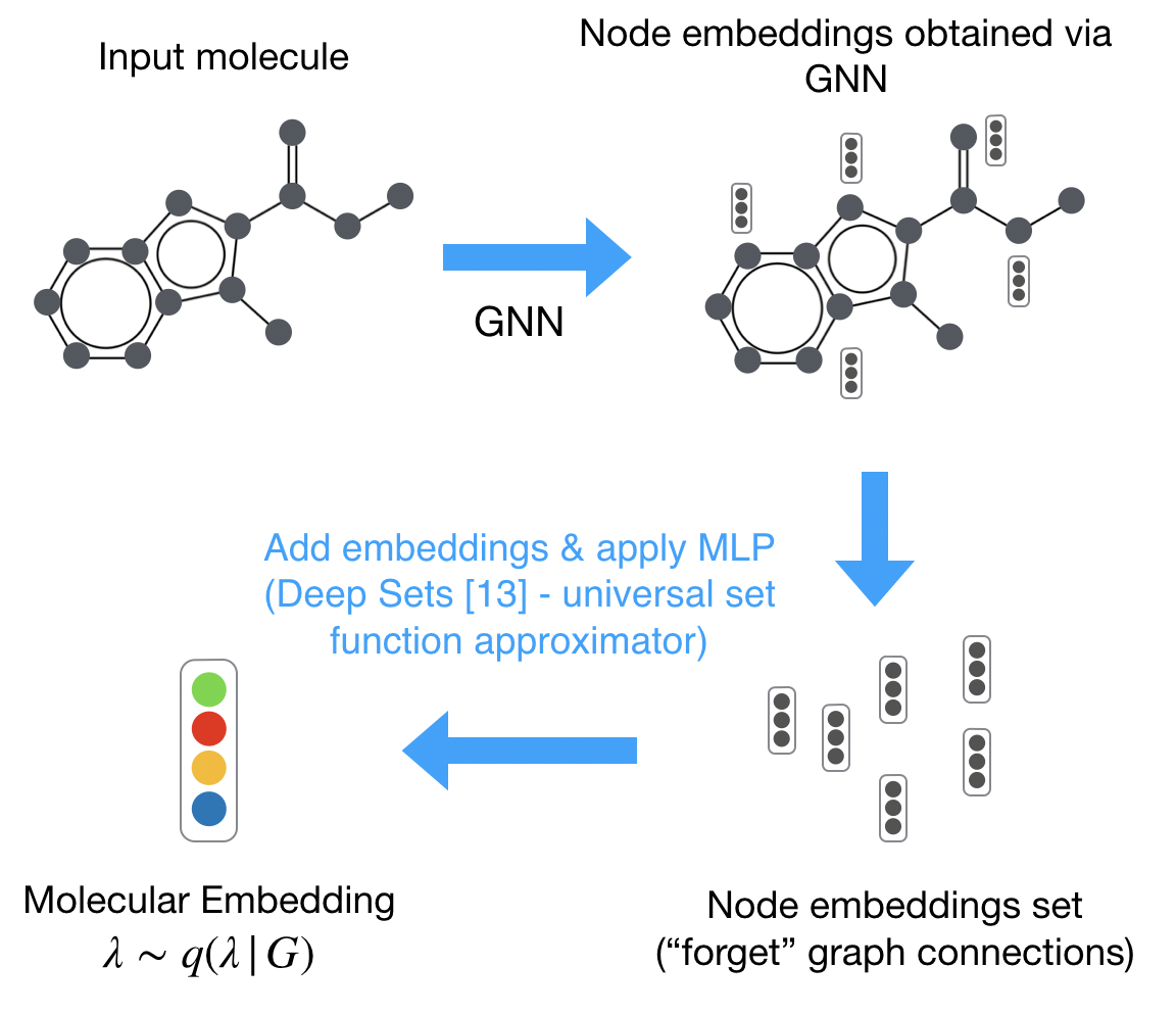
The molecular graph encoder uses a graph neural network to obtain node embeddings and then uses Deep Sets $\href{#13}{[13]}$ i.e. add embeddings & apply MLP on top, to obtain the molecular embedding.
Graph decoder - Issues #
Unfortunately, there is no straightforward way to generate a graph from a vector in one shot. Recall that the decoder should preserve permutation invariance w.r.t. to graph nodes, and ensure semantic validity of generated graphs.
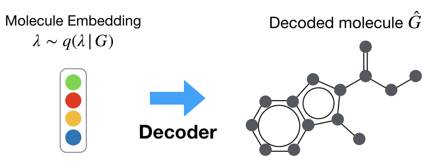
To explain some of the ideas to tackle this, we will make a small introduction to OT.
Optimal Transport intro #
Optimal transport (OT) studies the possible ways to morph a source measure $\mu$ into a target measure $\nu$, with special interest in the properties of the least costly way to achieve that and its efficient computation. Here we consider probability measures (with total volume $1$) and work with the Wasserstein distance and the Gromov-Wasserstein discrepancy.
For simplicity, we assume that the measures are uniform over the sets they are defined over (equal mass at each point), and represent these uniform measures with pointclouds e.g. if a pointcloud has $5$ points, each points carries $0.2$ mass.
Wasserstein distance #
Wasserstein (W) distance takes $2$ such pointclouds in the same metric measure space (but possibly of different number of points) and a cost function $c$ (e.g. L2), and finds the optimal way to morph one into the other.
\[\begin{equation} \mathcal{W}(\mathbf{X}, \mathbf{Y}) = \min_{\mathbf{T}\in {\mathcal{C}}_{\mathbf{X} \mathbf{Y}}} \sum_{ij} \mathbf{T}_{ij} \, c(\mathbf{x}_i, \mathbf{y}_j) \end{equation}\]where Transport plan $\mathbf{T}$ is a doubly stoachastic matrix, and $c(\mathbf{x}_i, \mathbf{y}_j)$ is the cost of transporting mass from $\mathbf{x}_i$ to $\mathbf{y}_j$.
Gromov-Wasserstein discrepancy #
Wasserstein distance needs a ground cost function $c$ to compare two points and thus can not be defined if those points are not defined on the same underlying space - or if we cannot preregister these spaces and define a cost between each pair of points of the two spaces.
Gromov-Wasserstein (GW) discrepancy addresses this limitation by using two matrices $\mathbf{A}$, $\mathbf{B}$ to quantify similiarity relationships within the two different metric measure spaces, $\mathcal{X}$ and $\mathcal{Y}$ respectively. This way we can relate graphs in terms of their structure e.g. comparing their shortest distance matrices.
\[\begin{equation} \mathcal{GW}(\mathbf{A}, \mathbf{B}) = \min_{\mathbf{T} \in \mathcal{C}_{\mathcal{X} \mathcal{Y}}} \sum\limits_{ij} \sum\limits_{kl} \mathbf{T}_{ij} \mathbf{T}_{kl} \, c(\mathbf{A}_{ik}, \mathbf{B}_{jl}) \end{equation}\]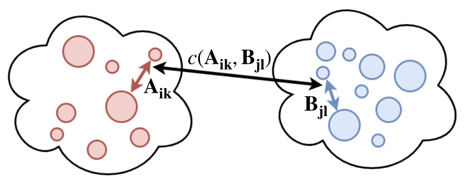
Graph decoder - Dictionary learning idea #
Xu H. $\href{#10}{[10]}$ proposed a generalization of dictionary learning for graphs. The idea is that every graph is expressed as a Fréchet mean (GW Barycenter) of learnable dictionary elements and $\lambda$ represents the weights of the dictionary elements.
![Dictionary learning for molecules, adapted from the idea in $\href{#10}{[10]}$](../../../assets/images/molgraphlearning/graph-decoder-dictionary-learning.png)
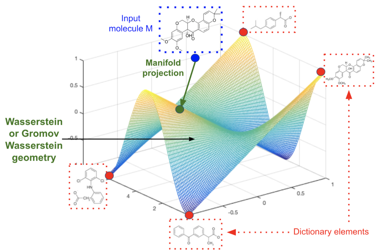
Caveats: GW Barycenter is hard to backpropagate through. Also we need to combine W and GW to decompose a graph with node and edge features and this has a lot of free parameters. We alternatively do something simpler and easier to train, but keep the idea of dictionary learning.
Graph decoder - Dictionary learning point clouds #
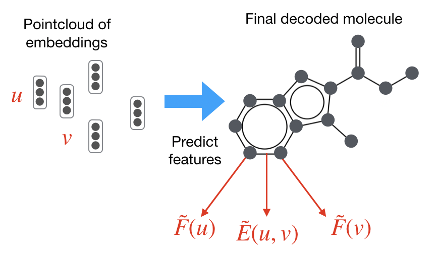
Instead of going from the molecular embedding to the molecule directly, we firstly generate a point cloud (node embedding set) from the embedding vector (Vec2Set) i.e. we perform dictionary learning on the pointcloud level, and then we predict the node and edge features.

In Vec2Set, we wish to generate a pointcloud from a vector $\lambda$ in a permutation invariant way. We use the dictionary learning idea discussed previously but on the node embedding level (therefore using the Wasserstein metric which is easier to backpropagate through than GW).
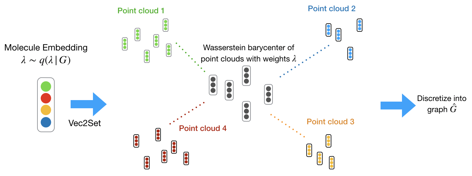
We use $\lambda$ as the weights and the point clouds / atoms / prototypes are free parameters to be learnt.
With pointclouds ${\{\mathbf{P}_i\}}_{i=1}^K$ and weights $\lambda \in \Delta^{K-1}$ we can compute the permutation invariant Wasserstein barycenter $\mathbf{B}$
\[arg\min_{\mathbf{B}}\sum_{i=1}^{K} \lambda_i \mathcal{W}(\mathbf{B}, \mathbf{P}_i)\]Regarding the number of nodes when decoding, we can memorize the number of input nodes and sample it on generation / optimization. This is equivalent to doing optimal transport based clustering, see $\href{#8}{[8]}$.
In practice this proves to be very slow and hard to train :( We resort to 2 simplified approaches.
SingleWB #
Assume the points in the point clouds have an apriori fixed matching. This is not too restrictive as these prototypes are free parameters and it doesn’t compromise the permutation invariance of the model. It just requires that all point clouds have the same size.
$arg\min_{\mathbf{B}}\sum_{i=1}^{K} \lambda_i \mathcal{W}(\mathbf{B}, \mathbf{P}_i)$ simplifies to $arg\min_{\mathbf{B}} \mathcal{W}(\mathbf{B}, \sum_{i=1}^{K} \lambda_i \mathbf{P}_i)$ since we don’t have to find the alignment between the point clouds, but only between their weighted average and the barycenter. Note that $\mathbf{B}$ can have a different number of points than the point cloud weighted average, hence the Wasserstein barycenter is still required.
Linear Interpolation #
We set $\mathbf{B} = \sum_k \lambda_k \mathbf{P}_k$ by adding the extra embeddings together. While this feels like cheating we will see that it matches the performance of SingleWB while converging much faster and being much more stable in training.
Non-dictionary learning mode #
We a predict fixed size point cloud from the latent representation. Then add extra embeddings together to form the point cloud of desired size.

So we got rid of OT with Linear Interpolation and Non-dictionary learning? At least on this step yes. However, we don’t know the alignment of the generated pointcloud and of the generated molecule with the initial one, so we’ll need OT later :)
Graph decoder - From pointcloud to discrete graph #
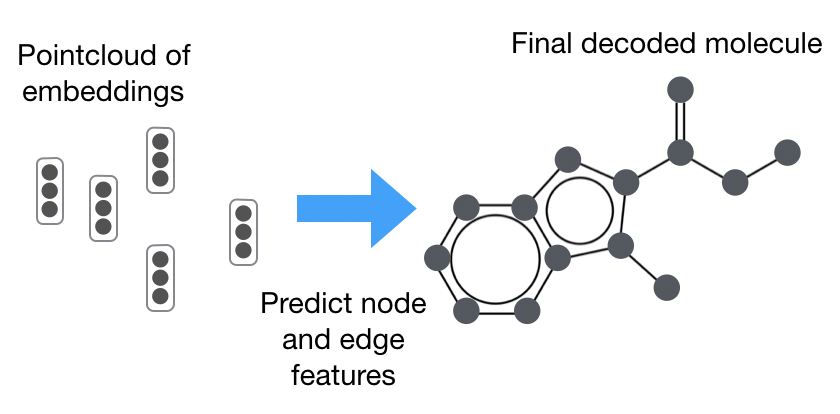
The following questions naturally arise:
How to predict features, i.e. go from node embedding set to a graph?
How to define a permutation invariant loss?
How to ensure the graph is a valid molecule?
1. How to predict features #
On each reconstructed embedding $u$, we apply a neural net $\tilde{F}(u)$ to predict a softmax distribution over the corresponding node feature vector (atom type). Similarly we apply a neural net $\tilde{E}(u,v)$ on pairs of embeddings to predict edges between two nodes.
2. How to define a permutation invariant loss? #
This is where OT comes back in to take care of permutation invariance. We match both nodes and edge features in a permutation invariant way using an OT pseudometric, the Fused Gromov-Wasserstein (FGW) $\href{#14}{[14]}$ discrepancy. We express the loss function $FGWLL_a(\mathbf{G}, \hat{\mathbf{G}})$, between input and reconstructed graphs $\mathbf{G}$ and $\hat{\mathbf{G}}$, using as cost functions $c_1$, $c_2$ the product of the log-likelihood of the target labels and a rescaling factor.


3. How to ensure the graph is a valid molecule? #
This proves to be one of the hardest parts of the pipeline. We explore $3$ methods.
- Argmax
- CRF for structured prediction on top of logits
- Penalty method to enforce discrete constraints
Argmax #
Argmax is pretty self-explanatory and used as a comparative baseline. We just pick the most probable label from each separate predicted feature distribution.
CRF for structured prediction on top of logits #
CRFs are undirected graphical models for structured prediction that model the conditional distribution $P(y | x)$, where $y$ are the output variables and $x$ the observed variables. The conditional distribution is modelled as the product of some factors, each of which depends on a subset of variables subject to normalization, $P(\mathbf{y}|\mathbf{x}) \propto \prod_f f(\mathbf{y}, \mathbf{x})$. In our case the observed variables are the logits and the output variables represent the final discretized reconstruction.
We can view the node and edge attributes as random variables which have some dependencies e.g. a Carbon node can have at most $4$ bonds. We aim to always predict valid molecules by performing structured prediction over the undirected CRF.
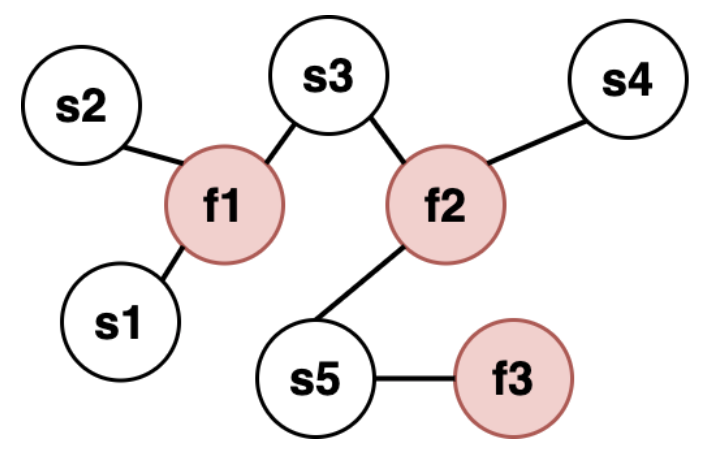
Belief propagation is an algorithm that can be used for inference in undirected graphical models. The algorithm is outlined below (initialize messages, iteratively update, compute marginals):
\[\begin{align*} &\mu_{f\rightarrow s}^t(x) = \sum\limits_{\mathbf{x}_f / x} f(\mathbf{x}_f) \prod\limits_{x'\in N(f) / s} \mu_{x'\rightarrow f}^{t-1}({\mathbf{x}_f}_{x'}) \\[3pt] &\mu_{s\rightarrow f}^t(x) = \prod\limits_{f'\in N(s) / f} \mu_{f'\rightarrow s}^{t-1}(x) \\[3pt] &\text{Marginal: } \mathbf P(s=i) \propto \prod\limits_{f\in N(s)} \mu_{f\rightarrow s}^{\textbf{T}}(i) \end{align*}\]The computational bottleneck of message passing lies in the $\mu_{f \rightarrow s}$ message. It has complexity as big as the cardinality of all random variables in the factor $f$.
To make this process differentiable we don’t require the factors (potentials) to be differentiable, we unroll the algorithm $\mathbf{T}$ times, place on top of network & learn parameters of factors via backpropagation. The factors are used to whitelist combinations of labels and to plug-in the logits e.g. a Carbon node will never have $2$ triple bonds but it’s very possible that is has $2$ double bonds.
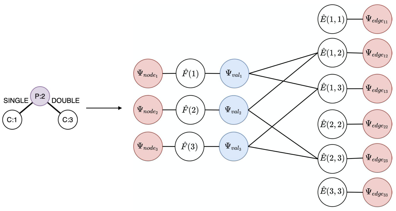
For observed variables $\tilde{F}(u)$ (node logits), $\tilde{E}(u, v)$ (edge logits), output variables $\hat{F}(u)$ (final nodes), $\hat{E}(u, v)$ (final edges), we define the following factors (think of them as the dependencies between the variables):
\[\begin{equation*} \Psi_{node_i}(\tilde{F}(i)) = exp(w_{node} \tilde{F}(i)) \end{equation*}\] \[\begin{equation*} \Psi_{edge_{ij}}(\tilde{E}(i, j)) = exp(w_{edge} \tilde{E}(i, j)) \end{equation*}\] \[\begin{equation*} \Psi_{val_i}(\hat{F}(i), \hat{E}(i, j) \, \forall j \in \{1..i-1,i+1,..n\}) = \begin{cases} \text{1} &\quad valency(\hat{F}(i)) \geq \sum\limits_j^n valency(\hat{E}(i, j))\\ \text{0} &\quad \text{otherwise}\\ \end{cases} \end{equation*}\] \[\begin{equation*} \Psi_{conn}(\hat{E}(i, j) \, \forall i, j: i < j \; i, j \in \{1..n\}) = \begin{cases} \text{1} &\quad \text{BFS from a node can reach all others}\\ \text{0} &\quad \text{otherwise}\\ \end{cases} \end{equation*}\]For $\mathbf{T}=10$ message passing iterations, connectivity is not tractable. Valency is tractable using pruning e.g. considering the top 6 most probable edges per node instead of all possible ones. Spoiler (or not): Valence enforcement works well but connectivity causes low validity overall with this method.
Penalty method #
The penalty method idea is to replace the constrained optimization problem, where the optimization constraints are discrete and non-differentiable (connectivity and valency over a discrete molecular graph), with an unconstrained problem which is formed by adding weighted penalty terms to the objective function. The idea in this context is to differentiably sample molecules from the predicted node/edge logits and add differentiable regularizing (penalty) terms to the training loss according to whether they satisfy the connectivity and valence constraints.
We can differentiably sample from logits using Gumbel softmax, softmax with temperature etc. Here we show only softmax with temperature, as we got more stable training with it. We sample from logits $z_i$ using a temperature $\tau$. The smaller $\tau$ is, the more one-hot are the post-softmax probabilities $y_i$.
\[y_i = \frac{exp(\frac{z_i}{\tau})}{\sum_j exp(\frac{z_j}{\tau})}\]Valence constraint penalty
Compute for each node $i$, the expected actual degree $E(i)$ (from the predicted bonds) and the expected maximum degree $M(i)$ (from the maximum valency of the predicted atom type). Also due to connectivity, the minimum degree is $1$.
\[penalty_{valence} = \sum_{\text{node }i} min(0,\, 1 - E(i)) + min(0, \, E(i) - M(i))\]Connectivity constraint penalty
The Laplacian matrix $\mathbf{L}$, is a matrix representation of the graph ($\mathbf{E}_{ij}$ edges of sampled graph).
\[\mathbf{L}_{kl} = \begin{cases} \sum_{m \neq k} \mathbf{E}_{km} & \text{, if } k = l,\\ -\mathbf{E}_{kl} & \text{, if } k \neq l\end{cases}\]Theorem$\href{#12}{[12]}$: $\mathbf{L}$ is symmetric and positive semidefinite. If $L + \frac{1}{N}\mathbf{1}_N\mathbf{1}_N^T$ is strictly positive definite then the graph is connected. This happens when its eigenvalues are positive.
\[penalty_{connectivity} = log(\frac{cap\_value ^ N}{\prod_i eig_i})\]All eigenvalues of $\mathbf{L}$ are non-negative and we want to penalize all reasonably small eigenvalues. We select a “cap value”, which indicates the maximum eigenvalue value that we penalize, by extracting the minimum eigenvalue from molecular datasets. We also don’t want the eigenvalues to be too small (since we use log) so we clamp them from below to $1e^{−8}$. The intuition is that the penalty will be 0 when the eigenvalues are all greater than the “cap value” and that we want an exponential loss for eigenvalues even slightly below the “cap value” - hence the log.
Euler constraint penalty
Since we work with 2D graphs we can use the Euler characteristic $|V| - |E| + |F| = 2$. Since $|F| = |Cycles| + 1$ and empirically $99.9\%$ of the molecules have up to $6$ cycles:
\[penalty_{euler} = min(0, |V| - 1 - |E|) + min(0, |E| - |V| - 5)\]Experiments #
We mainly use ChEMBL [7], which is a molecular dataset of 430K molecules, with a 80-10-10 split.
Validity #
We need to decode chemically valid molecules otherwise this method can’t be used in either property prediction, generation or optimization. Also we can’t measure chemical similarity between datasets if the molecules are invalid. Below we show our results with the $3$ different discretization strategies.
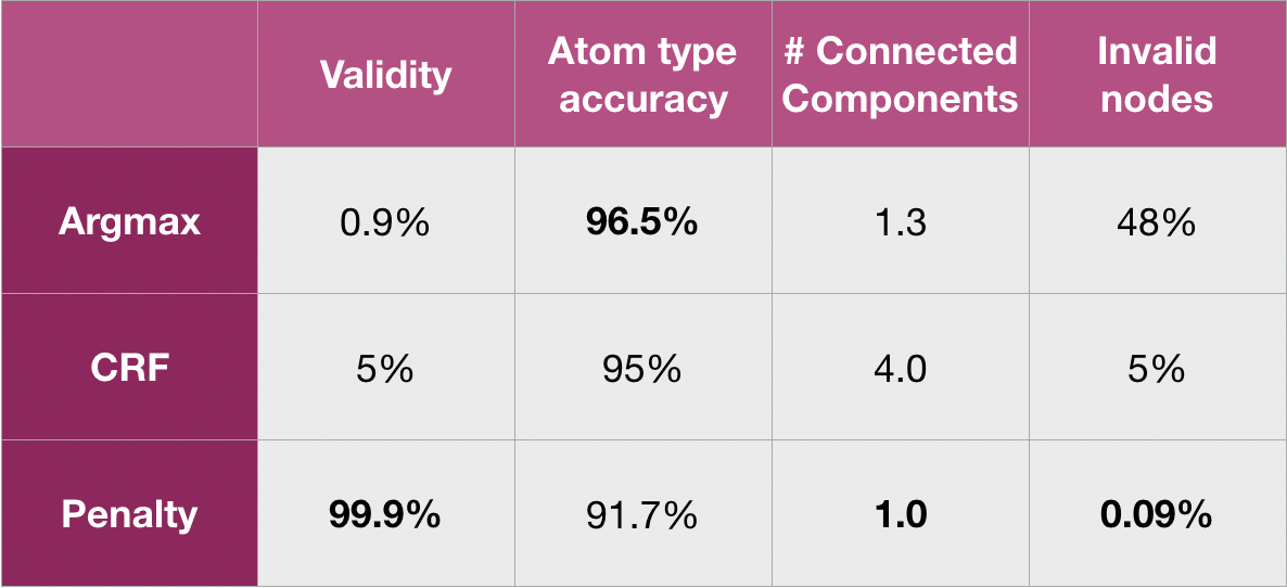
We see that with Argmax, we have the highest atom type accuracy (as expected, it has no regularizers), but have extremely low validity mainly caused by invalid valencies (invalid nodes). With the CRF, the validity is a bit higher as we manage to satisfy the valence constraints but get a lot of disconnected components. With the penalty method we manage to easily fit both and get $99.9\%$ validity with a little lower atom type accuracy. Comparing the proposed graph decoders: using the full Wasserstein barycenter doesn’t converge, SingleWB converges, Linear Interpolation converges the fastest, non-dictionary learning performs at most as good as Linear Interpolation when tweaked well.
Comparison with previous attempt #
We compare our apporach with Regularizing VAE $\href{#12}{[12]}$ where they attempt one-shot generation of valid molecules. They use the QM9 $\href{#27}{[27]}$ (small molecules dataset) and ZINC $\href{#9}{[9]}$ datasets.
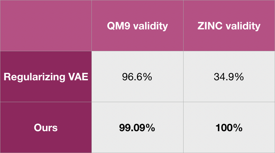
QM9 is a dataset with very small molecules (molecules have up to 9 nodes). ZINC is a more realistic dataset where Regularized VAE doesn’t perform that well. We also note that MolGAN $\href{#25}{[25]}$ is another previous attempt for generation on top of graph without autoregression. However, they also only report good results on QM9.
Tanimoto similarity #
Our models don’t perform greatly regarding Tanimoto similarity. In ChEMBL we achieve Tanimoto similarity of $10.1\%$ (chemical similarity of input and reconstructed molecules). We note that it’s easy for Tanimoto similarity to drop with the following example.
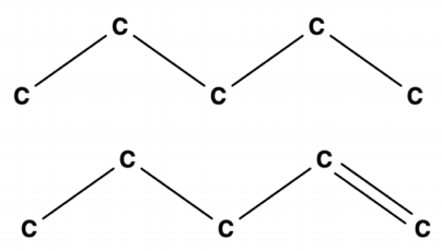
Even though we manage to reconstruct molecules, if they aren’t chemically similar to the input dataset our autoencoder is of little use to downstream tasks. We investigate what causes Tanimoto to drop, by cutting off a part of the pipeline.

Instead of collapsing to a single latent representation using Set2Vec we keep the node embeddings and decode directly. We remove therefore a part of the autoencoder (everything inside the black box). We know the node correspondences of the input and the output so we can also use L2 instead of FGW. Using FGW in this simplified setting (skipping everything inside the box), we still get $10\%$ Tanimoto similarity. Using L2 we get Tanimoto $> 50\%$. This means that GNN embeddings are not too weak since L2 succeeds in recovering the node and edge features from them. FGW is not strong enough to correlate the independent predictions of node and edge types.
Attempt at a downstream task #
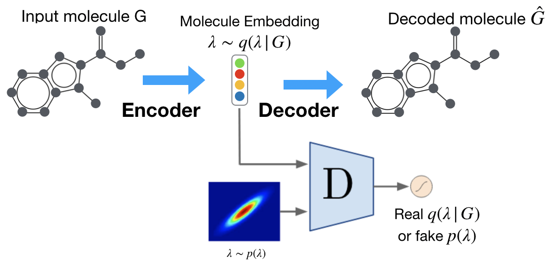
The FCD distance between the test dataset and a 1000 molecule generated dataset is too big (> 100). Our autoencoder has little usefulness due to the low Tanimoto similarity.
Future work idea - improving the Tanimoto similarity #
Instead of computing the FGW transport plan by solving an OT optimization problem, we can compute a cross attention matrix as described in $\href{#15}{[15]}$ between the two pointclouds (input and reconstructed). We can use that cross attention matrix as a differentiable transport plan in the FGW loss instead of using OT solvers.


Conclusion #
In this work we manage to generate semantically valid graphs in a one-shot isomorphically and permutation invariant way. We achieve $99.9\%$ validity on the ChEMBL dataset, much higher than previous attempts at the problem with highest validity $< 35\%$. We achieve this by enforcing discrete chemical constraints on graphs in a one-shot decoder. We observe, however, that the Tanimoto similarity of the decoded datasets and the input ones is not that high. Since we observe high node features accuracy ($91.7\%$) we attribute this to failing to learn the skeleton of the graph. This renders to be due to the OT loss we use, as it proves to be too weak to correlate the independent predictions of node and edge types. Due to the low Tanimoto similarity, this autoencoder doesn’t seem to be that useful in downstream tasks of property prediction, molecular generation and optimization. We believe that a way to improve the Tanimoto similarity could be to compute something similar to a transport matrix (replacing the FGW optimization problem), for example a differentiable cross attention matrix, which is easier to backpropagate through and can yield better results.
And that’s it! Thanks for reading this far! Too bad, the application of OT wasn’t that successful after all :) Feel free to reach out if you’re working on something similar or just want to talk about this.
Cited as:
@article{panayiotou2021molgraphlearn,
  title   = "Molecular graph learning in the Optimal Transport Geometry",
  author  = "Panayiotou, Panayiotis and Ganea, Octavian and Dragoi, Octav and Hofmann, Thomas",
  journal = "https://panpan2.github.io/",
  year    = "2021",
  url     = "https://panpan2.github.io/2021/04/20/molecular-graph-learning-in-the-optimal-transport-geometry"
}